

|
|
|
|
|
How to create a quantitation table
|
|
|
Introduction

|
The quantitation table contains all the necessary data, such
as the calibration curves, that are needed to quantitate one or
several components in a sample. This section describes how the quantitation
table is created.
|
|
|
|
|
How quantitation tables are created
|
Quantitation tables are created in the same way for both external
standard quantitation and for recovery calculations. They both use
absolute values of standard peak data.
For quantitation with internal standard, the peak sizes relative
to the size of the internal standard peak are used to create a calibration
curve.
|
|
|
|
|
Four process steps
|
The creation of the quantitation table can be divided into
four steps:
-
Standard data input
-
Component selection and definition
-
Peak identification
-
Calibration curve and quantitation table creation
|
|
|
|
|
Step 1 - How to input the standard data
|
The
table below describes how to input the standard data in the Evaluation module.
|
Step
|
Action
|
|
1
|
Select Quantitate:Edit
Quantitation Table:New on the menu bar.
Result: The New Quantitation Table dialog
box opens with the name of the active chromatogram displayed in
the Source chromatogram field.
|
|
2
|
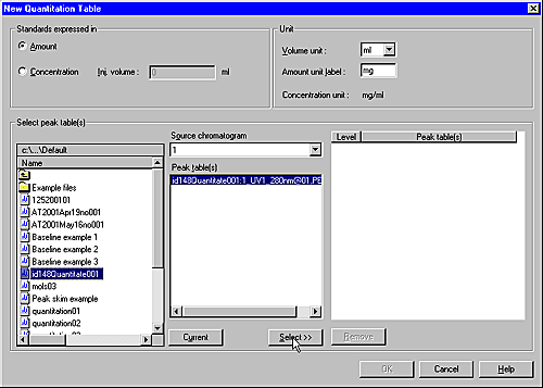
If desired, the standard can be expressed in Concentration instead of in Amount.
Note: The software
will always calculate both amount and concentration for the sample.
Note: This should
be the table for the highest or lowest concentration of the standard.
Result: The peak
table is added to the Level/Peak table(s) list.
|
|
3
|
-
The level
is automatically copied onto the list if it already was set in the
method. If so, continue with step 4.
-
If a level has not been
set, the Select Level dialog
box opens. Select 1 on the Level menu
and click OK.
|
|
4
|
Result: The peak
tables associated with this chromatogram are displayed on the Peak table(s) list.
|
|
5
|
Note: Increase the
level number for each new standard concentration in consecutive
order of decreasing or increasing concentration.
-
Click the Current button at any time to
return to the chromatogram that was active before you activated Quantitate.
-
Highlight unwanted tables on the list and click Remove.
-
Click OK to
finish the selection.
Result: The Define Component(s) dialog box
opens.
Continue to "Step 2, How to select and define components"
below this table.
|
|
|
|
|
|
Standard concentration levels
|
It
is useful to think of each level as an alias for a specific concentration
of the standard. You can incorporate up to 10 peak tables at each
level, prepared from runs repeated at the same concentration. Quantitate will later allocate
each with an incrementing suffix, e.g. 1:1, 1:2 etc.
|
|
|
|
|
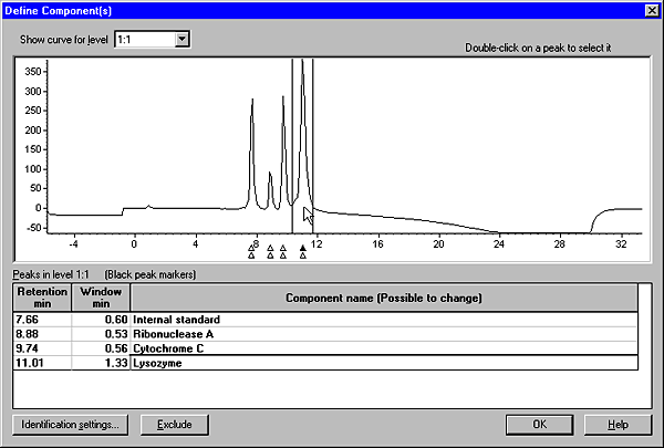
The Define Component(s) dialog box
|
The components that will be used to produce the calibration
curves are selected in the Define Component(s) dialog
box. Quantitate must be
able to identify these components on all levels. This dialog box
is used to set the criteria by which peaks are identified.
The illustration below shows the Define
Component(s) dialog box.
|
|
|
|
|
Examine the components
|
The Define Component(s) dialog
box initially displays the components from level 1:1, that is the
peak table from the highest or lowest concentration of the standard.
The Show curve for level list
is used to examine the curve for each standard run. The size of
the components are reduced or increased progressively as you select
levels further down on the list, which reflects the decreasing or
increasing concentration of the standard.
If an internal standard has been incorporated, its peak remains
about the same size on each level.
Peaks detected during the peak integration
Each component peak that was detected during the peak integration,
i.e. that is present in the peak table, is identified by a lower
triangle (black in level 1:1, green in other levels). There may
be different peaks detected for different levels. Upper triangles
will later identify the peaks that are selected for quantitation.
|
|
|
|
|
Step 2 - How to select and define components
|
The table
below describes how to select and define the components.
|
Step
|
Action
|
|
1
|
Select level 1:1 in the Show
curve for level list and click a peak.
Result: The peak
is highlighted in the table.
|
|
2
|
or
Result: The peak
is selected for quantitation, marked with an upper triangle and
"component no." is listed
as the Component name. The
selected peak is affected on all levels.
Note: More than
one peak can be selected to produce calibration curves for several
components.
|
|
3
|
Highlight the component name and type a new name.
|
|
4
|
Double-click the internal standard peak (if applicable)
and type a new name.
|
|
5
|
Continue to "Step 3, How to identify the peaks" below
this table.
|
|
|
|
|
|
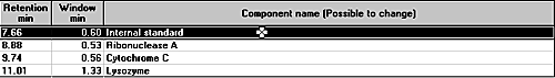
The Define component(s) peak table columns
|
The peak table within the Define
Component(s) dialog box has three columns:
-
The (absolute) Retention value of the component
in level 1:1.
-
The width of each component’s window. If you change
the width of the window by adjusting the cursor lines, this is reflected
in the Window column.
-
The Component name,
with the currently selected component highlighted.
|
|
|
|
|
Step 3 - How to identify the peaks
|
Description
When
a component is selected, vertical cursor lines show the current
identification window. The software uses this window to search for
peaks on other levels and in the sample runs. A peak found in the
window is assumed to be the component of interest. You can change
the limits by dragging a limit cursor line. Both cursor lines move
symmetrically so that the limits center on the component peak.
The window should be set wide enough to include peaks on the
other levels despite minor variations in retention volumes. However,
the window should also be narrow enough to exclude unwanted peaks
that will interfere with the quantitation.
Instruction
The table below describes how to adjust the window width for
the best results.
|
Step
|
Action
|
|
1
|
Drag the cursor lines to set the window to a suitable
width.
|
|
2
|
-
Use the Show curve for level menu to display
all levels and check that the width is suitable (the window width
is the same on all levels).
-
Click the lower green or black triangle to display
the actual retention for a peak.
|
|
3
|
Repeat steps 1 and 2 for all selected peaks.
Note: Overlapping
windows are not allowed.
|
|
4
|
If necessary, click the Identification
settings button to edit the settings. See "How to adjust
the identification settings" below this table.
|
|
5
|
Result: The Quantitation table dialog box
opens.
|
|
6
|
Continue to "Step 4, How to create a calibration curve
and a quantitation table" below this table.
|
|
|
|
|
|
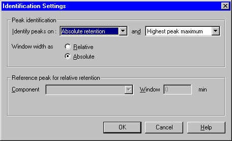
Identification settings
|
The criteria by which peaks are identified are set in the Identification Settings dialog
box. The criteria are valid for all the selected peaks in the Define Component(s) dialog box.
These settings also affect the information provided in the peak
table in the dialog box.
|
|
|
|
|
How to adjust the identification settings
|
Description
By
default, peaks are identified by their absolute retention values
and the highest peak maximum within the window. In most cases, it
is not necessary to change these default settings. Peak identification
by absolute retention works well when there has been little or no
drift in retention between successive runs of the standard. Quantitate
will find corresponding peaks in these successive runs providing
any drift in retention does not move a peak outside the peak window.
Instruction
If
you have drifting retention that makes peak identification difficult
you can choose to identify peaks according to their position relative
to a reference peak. The table below describes how to adjust the
identification settings in the Define Component(s) dialog
box.
|
Step
|
Action
|
|
1
|
Identify a component peak that can be used as the reference.
Note: Choose a peak
that is well separated from any other peaks. This enables the window
to be set relatively wide and the system can accommodate a larger
drift in retention value.
|
|
2
|
Click Identification Settings.
Result: The Identification Settings dialog
box opens.
See "How to identify peaks within a window" below.
|
|
3
|
Select Relative retention on
the Identify peaks on droplist.
(See "Absolute and Relative window width" below)
|
|
4
|
Scroll down the Component menu
and select the component to be used as the reference peak.
|
|
5
|
Note: Set the width
fairly wide to accommodate a larger drift in the retention value.
Make sure that there are no other large peaks within the window.
Result: A column
for the relative retention is added in the peak table, Ret/Ref.
The column displays the value of each component relative to the
retention value of the reference component. This reference component
is marked Ref. in the Window% column. The Window% column shows the window
width for each peak expressed as a percentage of its relative retention
value.
|
|
|
|
|
|
How to identify peaks within a window
|
Quantitate must be advised of
how the peaks are to be identified if any of the windows includes
more than one peak. The second droplist in the Peak identification field of the Identification Settings dialog
box offers the following options:
-
Highest peak maximum (default).
-
Closest to retention,
i.e. closest to the center of the window (see the retention column
in the peak table.)
-
Maximum peak area.
Examine the nature of the peaks enclosed by the window and
select the option that differs between the wanted and the unwanted
peaks. Use Closest to retention if there
are large peaks from components that are not going to be quantitated.
Note: The selection
applies to all peaks, even the internal standard and reference if used.
|
|
|
|
|
Absolute and Relative window width
|
When the Peak identification is
set to Absolute retention,
the peak window width can be displayed as Absolute or Relative. Select the appropriate
button in the Identification Settings dialog
box.
If Peak identification is
set to Relative retention, Window is set automatically to Relative except for the reference
peak.
|
|
|
|
|
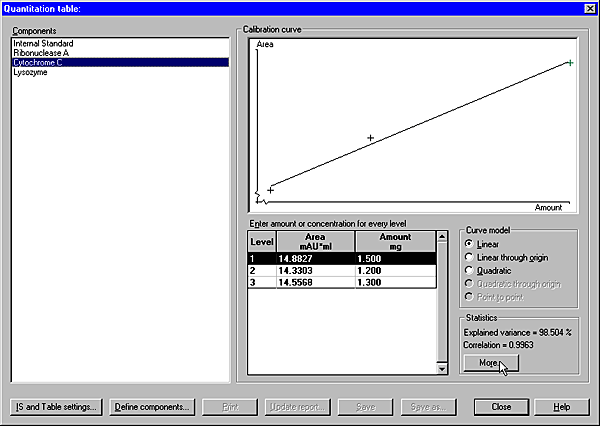
Step 4 - How to create a calibration curve and a quantitation table
|
When
the component selection and identification settings are completed
(see Step 3), the Quantitation table dialog
box is opened:
The
table below describes how to enter data for the standards and create
a quantitation table and a calibration curve.
|
Step
|
Action
|
|
1
|
|
|
2
|
-
Verify that
the selected components in the Components list
are correct.
If an internal
standard is used, the related component is labelled (IS).
If relative retention has been used, the reference
component is labelled (Ref).
|
|
3
|
Note: Do not select
an internal standard component (if available) as the amount for
this has already been entered and does not change between the levels.
Note: This is the
amount corresponding to the injected volume, not the total amount
used when the standard level was prepared.
|
|
4
|
Click the Curve model radio
button for the best curve model:
Result: The curve
is displayed in the Calibration curve window. Each
component level is labelled with crosses. If more than one run has
been performed for any level, all points in that level will be shown.
The average of these points is calculated and this value is used to
produce the calibration curve.
|
|
5
|
Repeat steps 3 and 4 for all the remaining components.
Result: The quantitation
table is complete with a calibration curve for each component.
|
|
6
|
or
Result: The Save quantitation table dialog
box opens.
Note: The Save button is used to save updates
in an existing quantitation table. However, this will overwrite
the original table. You might prefer to use Save
as and create a new name for the edited table to preserve
the original.
|
|
7
|
|
|
|
|
|
|
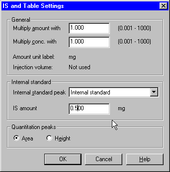
How to select an Internal Standard
|
The
table below describes how to select an internal standard in the Quantitation table dialog box.
|
Step
|
Action
|
|
1
|
Click the IS and Table
settings button.
Result: The IS and Table Settings dialog box
opens.
The illustration below shows the IS
and Table Settings dialog box with an Internal standard selected.
|
|
2
|
Type the amount and concentration multipliers in the General field.
Note: These values
are normally set to 1. See remarks below.
|
|
3
|
Select the internal standard component on the Internal standard peak droplist.
Note: The default
option is Not selected,
which is used for external standard quantitation and measurements
of the recovery factor.
|
|
4
|
Type the injected internal standard amount for the
standard and sample runs in the IS
amount text box.
|
|
5
|
Select if the quantitation will be based on Area (default) or Height in the Quantitation peaks field.
Note: Select Height if the peaks are not completely
separated from those of other components.
|
|
6
|
Click OK.
|
Note: The amount
and concentration of the sample are multiplied by the multiplier values
when the calibration curve is applied to a sample. Change the default
values if you want to determine the amount or concentration in the
starting volume of the sample instead of in the injected volume
of the sample.
|
|
|
|
|
Quantitation statistics
|
The Statistics field in the Quantitation table dialog box
displays the Correlation and Explained variance values when
available.
Click the More button
to open the Statistics dialog
box for a complete display of available data.
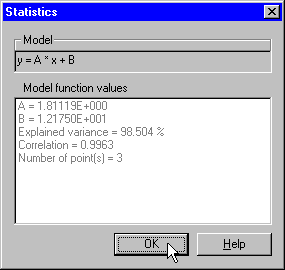
Statistical reference values
Note that the value is usually rather high even for poor models.
A value of 90% indicates a very poor model.
The explained variance is not shown for curve models that
are drawn through the origin.
Note: If the point-to-point
curve model is selected, no statistics are available.
|
|
|
|
2005-06-15
|
|
|