

|
|
Smoothing algorithms
|
|
|
Introduction

|
This section describes how the smoothing functions are calculated.
Choose Operations:Smooth in
the Evaluation module to
view and edit the options.
|
|
|
|
|
Moving Average
|
The
table below describes the process when the Moving
Average smoothing algorithm is used.
|
Stage
|
Description
|
|
1
|
For each data point in the source curve, the processed
curve is calculated as the average of the data points within a window
centered on the source data point.
|
|
2
|
When the source point is less than half the window
size from the beginning of the end of the curve, the average is
calculated symmetrically round the source point over as many data
points as possible.
|
Note: The filter
algorithm only accepts odd integer parameter values between 1 and 151.
If an even number has been given, it is incremented by one (1).
|
|
|
|
|
Autoregressive
|
The
table below describes the process when the Autoregressive smoothing
algorithm is used:
|
Stage
|
Description
|
|
1
|
The first data point in the source curve is copied
to the processed curve.
|
|
2
|
For each subsequent data point, the previous processed
point is multiplied with the parameter value and added to the current
source data point.
|
|
3
|
The result is then divided by the parameter value plus
1 according to the following formulae:
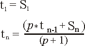
Where:
tn = current processed point.
tn-1 = previous processed point.
Sn = current source point.
p = smoothing parameter value.
Note: If you increase
the parameter value, the smoothing effect is also increased.
|
Note: The filter
algorithm only accepts integer parameter values between 1 and 25.
|
|
|
|
|
Median
|
The
table below describes the process when the Median smoothing
algorithm is used.
|
Stage
|
Description
|
|
1
|
For each data point in the source curve, the processed
curve is calculated as the median of the data points within a window
centered on the source data point.
|
|
2
|
When the source point is less than half the window
size from the beginning of the end of the curve, the median is calculated
symmetrically round the source point over as many data points as
possible.
-
If you increase the
window width, the smoothing effect is also increased.
-
To completely remove a noise spike, the window width
should in effect be slightly more than twice the width of the spike.
|
Note: The filter
algorithm only accepts odd integer parameter values between 1 and 151.
If an even number has been given, it is incremented by one.
|
|
|
|
|
Savitzky-Golay
|
The
table below describes the process when the Savitzky-Golay smoothing
algorithm is used.
|
Stage
|
Description
|
|
1
|
The algorithm is based on performing a least squares
linear regression fit of a polynominal of degree k over at least
k+1 data points around each point in the curve to smoothen the data.
The derivate is the derivate of the fitted polynominal at
each point.
The calculation uses a convolution formalism to calculate
1st through 9th derivatives.
|
|
2
|
The calculation is performed with the data in low X
to high X order.
If the input trace goes from low to high, it is reversed for
the calculation and is re-reversed afterwards.
|
Note: See Gorry,
Peter A, General Least-Squares Smoothing and Differentation by the
Convolution (Savitsky-Golay) Method (Analytical Chemistry 1990,
Volume 62, 570-573) for more information on the Savitzky-Golay algorithm.
|
|
|
|
2005-06-15
|
|
|